To get a better handle on custom epi_workflow()s, lets
recreate and then modify the example of four_week_ahead
from the landing page
training_data <- covid_case_death_rates |>
  filter(time_value <= forecast_date, geo_value %in% used_locations)
four_week_ahead <- arx_forecaster(
  training_data,
  outcome = "death_rate",
  predictors = c("case_rate", "death_rate"),
  args_list = arx_args_list(
    lags = list(c(0, 1, 2, 3, 7, 14), c(0, 7, 14)),
    ahead = 4 * 7,
    quantile_levels = c(0.1, 0.25, 0.5, 0.75, 0.9)
  )
)
four_week_ahead$epi_workflow
#>
#> ══ Epi Workflow [trained] ═══════════════════════════════════════════════════
#> Preprocessor: Recipe
#> Model: linear_reg()
#> Postprocessor: Frosting
#>
#> ── Preprocessor ─────────────────────────────────────────────────────────────
#>
#> 6 Recipe steps.
#> 1. step_epi_lag()
#> 2. step_epi_lag()
#> 3. step_epi_ahead()
#> 4. step_naomit()
#> 5. step_naomit()
#> 6. step_training_window()
#>
#> ── Model ────────────────────────────────────────────────────────────────────
#>
#> Call:
#> stats::lm(formula = ..y ~ ., data = data)
#>
#> Coefficients:
#>       (Intercept)    lag_0_case_rate    lag_1_case_rate    lag_2_case_rate
#>        -0.0060191          0.0004648          0.0021793          0.0004928
#>   lag_3_case_rate    lag_7_case_rate   lag_14_case_rate   lag_0_death_rate
#>         0.0007806         -0.0021676          0.0018002          0.4258788
#>  lag_7_death_rate  lag_14_death_rate
#>         0.1632748         -0.1584456
#>
#> ── Postprocessor ────────────────────────────────────────────────────────────
#>
#> 5 Frosting layers.
#> 1. layer_predict()
#> 2. layer_residual_quantiles()
#> 3. layer_add_forecast_date()
#> 4. layer_add_target_date()
#> 5. layer_threshold()
#>
Anatomy of an epi_workflow
An epi_workflow() is an extension of a
workflows::workflow() to handle panel data and
post-processing. It consists of 3 components, shown above:
- Preprocessor: transform the data before model training and
prediction, such as convert counts to rates, create smoothed columns, or
any of the
recipes steps. Think of it as a more flexible
formulathat you would pass tolm():y ~ x1 + log(x2) + lag(x1, 5). The above model has 6 of these steps. In general, there are 2 broad classes of transformation that recipes handles:- Transforms of both training and test data that are always applied. Examples include taking the log of a variable, leading or lagging, filtering out rows, handling dummy variables, calculating growth rates, etc.
- Operations that fit parameters during training to apply during prediction, such as centering by the mean. This is a major benefit of recipes, since it prevents data leakage, where information about the test/predict time data “leaks” into the parameters. However, the main mechanism we rely on to prevent data leakage is proper backtesting. For the case of centering, we need to store the mean of the predictor from the training data and use that value on the prediction data rather than accidentally calculating the mean of the test predictor for centering.
- Trainer: use a parsnip model to train a model on data, resulting in a fitted model object. Examples include linear regression, quantile regression, or any parsnip engine. Parsnip serves as a front-end that abstracts away the differences in interface between a wide collection of statistical models.
- Postprocessor: unique to this package, and used to format and modify
the prediction after the model has been fit. Each operation is a
layer_, and the stack of layers is known asfrosting(), continuing the metaphor of baking a cake established in the recipe. Some example operations include:- generate quantiles from purely point-prediction models,
- undo operations done in the steps, such as convert back to counts from rates
- threshold so the forecast doesn’t include negative values
- generally adapt the format of the prediction to it’s eventual use.
Recreating four_week_ahead in an
epi_workflow()
To be able to extend this beyond what arx_forecaster()
itself will let us do, we first need to understand how to recreate it
using a custom epi_workflow().
To use a custom workflow, there are a couple of steps:
- define the
epi_recipe(), which contains the preprocessing steps - define the
frosting()which contains the post-processing layers - Combine these with a trainer such as
quantile_reg()into anepi_workflow(), which we can then fit on the training data -
fit()the workflow on some data - grab the right prediction data using
get_test_data()and apply the fit data to generate a prediction
Define the epi_recipe()
To do this, we’ll first take a look at the steps as they’re found in
four_week_ahead:
hardhat::extract_recipe(four_week_ahead$epi_workflow)
#>
#> ── Epi Recipe ───────────────────────────────────────────────────────────────
#>
#> ── Inputs
#> Number of variables by role
#> raw:        2
#> geo_value:  1
#> time_value: 1
#>
#> ── Training information
#> Training data contained 856 data points and no incomplete rows.
#>
#> ── Operations
#> 1. Lagging: case_rate by 0, 1, 2, 3, 7, 14 | Trained
#> 2. Lagging: death_rate by 0, 7, 14 | Trained
#> 3. Leading: death_rate by 28 | Trained
#> 4. • Removing rows with NA values in: lag_0_case_rate, ... | Trained
#> 5. • Removing rows with NA values in: ahead_28_death_rate | Trained
#> 6. • # of recent observations per key limited to:: Inf | Trained
So there are 6 steps we will need to recreate. One thing to note
about the extracted recipe is that it has already been trained; for
steps such as recipes::step_BoxCox() which have parameters,
this means that their parameters have been calculated. Before defining
steps, we need to create an epi_recipe() to hold them
four_week_recipe <- epi_recipe(
  covid_case_death_rates |>
    filter(time_value <= forecast_date, geo_value %in% used_locations)
)
The data here, covid_case_death_rates doesn’t strictly
need to be the actual dataset on which you are going to train. However,
it should have the same columns and the same metadata, such as
as_of or other_keys; it is typically easiest
to just use the training data itself.
Then we add each step via pipes; in principle the order matters,
though for this recipe only step_epi_naomit() and
step_training_window() depend on the steps before them:
four_week_recipe <- four_week_recipe |>
  step_epi_lag(case_rate, lag = c(0, 1, 2, 3, 7, 14)) |>
  step_epi_lag(death_rate, lag = c(0, 7, 14)) |>
  step_epi_ahead(death_rate, ahead = 4 * 7) |>
  step_epi_naomit() |>
  step_training_window()
One thing to note: we only added 5 steps here because
step_epi_naomit() is actually a wrapper around adding 2
base step_naomit()s, one for all_predictors()
and one for all_outcomes(), differing in their treatment at
predict time.
step_epi_lag() and step_epi_ahead() both
accept tidy syntax, so if for example we wanted the same lags for both
case_rate and death_rate, we could have done
step_epi_lag(ends_with("rate"), lag = c(0, 7, 14)).
In general for the recipes package, steps assign
roles, such as predictor and outcome to
columns, either by adding new columns or adjusting existing ones.
step_epi_lag() for example, creates a new column for each
lag with the name lag_x_column_name and assigns them as
predictors, while step_epi_ahead() creates
ahead_x_column_name columns and assigns them as
outcomes.
One way to inspect the roles assigned is to use
prep():
prepped <- four_week_recipe |> prep(training_data)
prepped$term_info |> print(n = 14)
#> # A tibble: 14 × 4
#>    variable            type    role       source
#>    <chr>               <chr>   <chr>      <chr>
#>  1 geo_value           nominal geo_value  original
#>  2 time_value          date    time_value original
#>  3 case_rate           numeric raw        original
#>  4 death_rate          numeric raw        original
#>  5 lag_0_case_rate     numeric predictor  derived
#>  6 lag_1_case_rate     numeric predictor  derived
#>  7 lag_2_case_rate     numeric predictor  derived
#>  8 lag_3_case_rate     numeric predictor  derived
#>  9 lag_7_case_rate     numeric predictor  derived
#> 10 lag_14_case_rate    numeric predictor  derived
#> 11 lag_0_death_rate    numeric predictor  derived
#> 12 lag_7_death_rate    numeric predictor  derived
#> 13 lag_14_death_rate   numeric predictor  derived
#> 14 ahead_28_death_rate numeric outcome    derived
The way to inspect the columns created is by using
bake() on the resulting recipe:
four_week_recipe |>
  prep(training_data) |>
  bake(training_data)
#> An `epi_df` object, 800 x 14 with metadata:
#> * geo_type  = state
#> * time_type = day
#> * as_of     = 2023-03-10
#>
#> # A tibble: 800 × 14
#>   geo_value time_value case_rate death_rate lag_0_case_rate lag_1_case_rate
#> * <chr>     <date>         <dbl>      <dbl>           <dbl>           <dbl>
#> 1 ca        2021-01-14     108.       1.22            108.            111.
#> 2 ma        2021-01-14      88.7      0.893            88.7            92.0
#> 3 ny        2021-01-14      82.4      0.969            82.4            84.9
#> 4 tx        2021-01-14      74.9      1.05             74.9            75.0
#> 5 ca        2021-01-15     104.       1.21            104.            108.
#> 6 ma        2021-01-15      83.3      0.908            83.3            88.7
#> # ℹ 794 more rows
#> # ℹ 8 more variables: lag_2_case_rate <dbl>, lag_3_case_rate <dbl>, …
This is also useful for debugging malfunctioning pipelines; if you
define four_week_recipe only up to the step that is
misbehaving, you can get a partial evaluation to see the exact data the
step is being applied to. It also allows you to see the exact data that
the parsnip model is fitting on.
Define the frosting()
Since the post-processing frosting layers1 are unique to this
package, to inspect them we use extract_frosting() from
epipredict:
epipredict::extract_frosting(four_week_ahead$epi_workflow)
#>
#> ── Frosting ─────────────────────────────────────────────────────────────────
#>
#> ── Layers
#> 1. Creating predictions: "<calculated>"
#> 2. Resampling residuals for predictive quantiles: "<calculated>"
#> 3. quantile_levels 0.1, 0.25, 0.5, 0.75, 0.9
#> 4. Adding forecast date: "2021-08-01"
#> 5. Adding target date: "2021-08-29"
#> 6. Thresholding predictions: dplyr::starts_with(".pred") to [0, Inf)
The above gives us detailed descriptions of the arguments to the
functions named above in the postprocessor of
four_week_ahead$epiworkflow. Creating the layers is a
similar process, except with frosting instead of a recipe2:
four_week_layers <- frosting() |>
  layer_predict() |>
  layer_residual_quantiles(quantile_levels = c(0.1, 0.25, 0.5, 0.75, 0.9)) |>
  layer_add_forecast_date() |>
  layer_add_target_date() |>
  layer_threshold()
Most layers will work for any engine or steps;
layer_predict() you will want to call in every case. There
are a couple of layers, however, which depend on whether the engine used
predicts quantiles or point estimates.
The layers that are only supported by point estimate engines (such as
linear_reg()) are
-
layer_residual_quantiles(): the preferred method of generating quantiles for non-quantile models, it uses the error residuals of the engine. This will work for most parsnip engines. -
layer_predictive_distn(): alternate method of generating quantiles, it uses an approximate parametric distribution. This will work for linear regression specifically.
TODO check this
On the other hand, the layers that are only supported by quantile
estimating engines (such as quantile_reg()) are
-
layer_quantile_distn(): adds the specified quantiles. If they differ from the ones actually fit, they will be interpolated and/or extrapolated. -
layer_point_from_distn(): this adds the median quantile as a point estimate, and should be called afterlayer_quantile_distn()if called at all.
Fitting an epi_workflow()
Given that we now have a recipe and some layers, we need to assemble the workflow:
four_week_workflow <- epi_workflow(
  four_week_recipe,
  linear_reg(),
  four_week_layers
)
And fit it to recreate four_week_ahead$epi_workflow
fit_workflow <- four_week_workflow |> fit(training_data)Predicting
To do a prediction, we need to first narrow the dataset down to the relevant datapoints:
relevant_data <- get_test_data(
  four_week_recipe,
  training_data
)
With a fit workflow and test data in hand, we can actually make our predictions:
fit_workflow |> predict(relevant_data)
#> An `epi_df` object, 4 x 6 with metadata:
#> * geo_type  = state
#> * time_type = day
#> * as_of     = 2023-03-10
#>
#> # A tibble: 4 × 6
#>   geo_value time_value .pred .pred_distn forecast_date target_date
#>   <chr>     <date>     <dbl>   <qtls(5)> <date>        <date>
#> 1 ca        2021-08-01 0.341     [0.341] 2021-08-01    2021-08-29
#> 2 ma        2021-08-01 0.163     [0.163] 2021-08-01    2021-08-29
#> 3 ny        2021-08-01 0.196     [0.196] 2021-08-01    2021-08-29
#> 4 tx        2021-08-01 0.404     [0.404] 2021-08-01    2021-08-29
Note that if we had simply plugged training_data into
predict() we still get predictions:
fit_workflow |> predict(training_data)
#> An `epi_df` object, 800 x 6 with metadata:
#> * geo_type  = state
#> * time_type = day
#> * as_of     = 2023-03-10
#>
#> # A tibble: 800 × 6
#>   geo_value time_value .pred .pred_distn forecast_date target_date
#>   <chr>     <date>     <dbl>   <qtls(5)> <date>        <date>
#> 1 ca        2021-01-14 0.997     [0.997] 2021-08-01    2021-08-29
#> 2 ma        2021-01-14 0.835     [0.835] 2021-08-01    2021-08-29
#> 3 ny        2021-01-14 0.868     [0.868] 2021-08-01    2021-08-29
#> 4 tx        2021-01-14 0.581     [0.581] 2021-08-01    2021-08-29
#> 5 ca        2021-01-15 0.869     [0.869] 2021-08-01    2021-08-29
#> 6 ma        2021-01-15 0.830      [0.83] 2021-08-01    2021-08-29
#> # ℹ 794 more rows
The resulting tibble is 800 rows long, however. This produces
forecasts for not just the actual forecast_date, but for
every day in the dataset it has enough data to actually make a
prediction. To narrow this down, we could filter to rows where the
time_value matches the forecast_date:
fit_workflow |>
  predict(training_data) |>
  filter(time_value == forecast_date)
#> An `epi_df` object, 4 x 6 with metadata:
#> * geo_type  = state
#> * time_type = day
#> * as_of     = 2023-03-10
#>
#> # A tibble: 4 × 6
#>   geo_value time_value .pred .pred_distn forecast_date target_date
#>   <chr>     <date>     <dbl>   <qtls(5)> <date>        <date>
#> 1 ca        2021-08-01 0.341     [0.341] 2021-08-01    2021-08-29
#> 2 ma        2021-08-01 0.163     [0.163] 2021-08-01    2021-08-29
#> 3 ny        2021-08-01 0.196     [0.196] 2021-08-01    2021-08-29
#> 4 tx        2021-08-01 0.404     [0.404] 2021-08-01    2021-08-29
This can be useful for cases where get_test_data()
doesn’t pull sufficient data.
Extending four_week_ahead
There are many ways we could modify four_week_ahead; one
simple modification would be to include a growth rate estimate as part
of the model. Another would be to convert from rates to counts, for
example if that were the preferred prediction format. Another would be
to include a time component to the prediction (useful if we expect there
to be a strong seasonal component).
Growth rate
One feature that may potentially improve our forecast is looking at the growth rate
growth_rate_recipe <- epi_recipe(
  covid_case_death_rates |>
    filter(time_value <= forecast_date, geo_value %in% used_locations)
) |>
  step_epi_lag(case_rate, lag = c(0, 1, 2, 3, 7, 14)) |>
  step_epi_lag(death_rate, lag = c(0, 7, 14)) |>
  step_epi_ahead(death_rate, ahead = 4 * 7) |>
  step_epi_naomit() |>
  step_growth_rate(death_rate) |>
  step_training_window()
Inspecting the newly added column:
growth_rate_recipe |>
  prep(training_data) |>
  bake(training_data) |>
  select(
    geo_value, time_value, case_rate,
    death_rate, gr_7_rel_change_death_rate
  )
#> An `epi_df` object, 800 x 5 with metadata:
#> * geo_type  = state
#> * time_type = day
#> * as_of     = 2023-03-10
#>
#> # A tibble: 800 × 5
#>   geo_value time_value case_rate death_rate gr_7_rel_change_death_rate
#>   <chr>     <date>         <dbl>      <dbl>                      <dbl>
#> 1 ca        2021-01-14     108.       1.22                          NA
#> 2 ma        2021-01-14      88.7      0.893                         NA
#> 3 ny        2021-01-14      82.4      0.969                         NA
#> 4 tx        2021-01-14      74.9      1.05                          NA
#> 5 ca        2021-01-15     104.       1.21                          NA
#> 6 ma        2021-01-15      83.3      0.908                         NA
#> # ℹ 794 more rows
And the role:
prepped <- growth_rate_recipe |>
  prep(training_data)
prepped$term_info |> filter(grepl("gr", variable))
#> # A tibble: 1 × 4
#>   variable                   type    role      source
#>   <chr>                      <chr>   <chr>     <chr>
#> 1 gr_7_rel_change_death_rate numeric predictor derived
To demonstrate the changes in the layers that come along with it, we
will use quantile_reg() as the model, which requires
changing from layer_residual_quantiles() to
layer_quantile_distn() and
layer_point_from_distn():
growth_rate_layers <- frosting() |>
  layer_predict() |>
  layer_quantile_distn(
    quantile_levels = c(0.1, 0.25, 0.5, 0.75, 0.9)
  ) |>
  layer_point_from_distn() |>
  layer_add_forecast_date() |>
  layer_add_target_date() |>
  layer_threshold()

growth_rate_workflow <- epi_workflow(
  growth_rate_recipe,
  quantile_reg(quantile_levels = c(0.1, 0.25, 0.5, 0.75, 0.9)),
  growth_rate_layers
)

relevant_data <- get_test_data(
  growth_rate_recipe,
  training_data
)
gr_fit_workflow <- growth_rate_workflow |> fit(training_data)
gr_predictions <- gr_fit_workflow |>
  predict(relevant_data) |>
  filter(time_value == forecast_date)
Plot
Plotting the result; this is reusing some code from the landing page to print the forecast date.
forecast_date_label <-
  tibble(
    geo_value = rep(used_locations, 2),
    .response_name = c(rep("case_rate", 4), rep("death_rate", 4)),
    dates = rep(forecast_date - 7 * 2, 2 * length(used_locations)),
    heights = c(rep(150, 4), rep(0.30, 4))
  )

result_plot <- autoplot(
  object = gr_fit_workflow,
  predictions = gr_predictions,
  plot_data = covid_case_death_rates |>
    filter(geo_value %in% used_locations, time_value > "2021-07-01")
) +
  geom_vline(aes(xintercept = forecast_date)) +
  geom_text(
    data = forecast_date_label %>% filter(.response_name == "death_rate"),
    aes(x = dates, label = "forecast\ndate", y = heights),
    size = 3, hjust = "right"
  ) +
  scale_x_date(date_breaks = "3 months", date_labels = "%Y %b") +
  theme(axis.text.x = element_text(angle = 90, hjust = 1))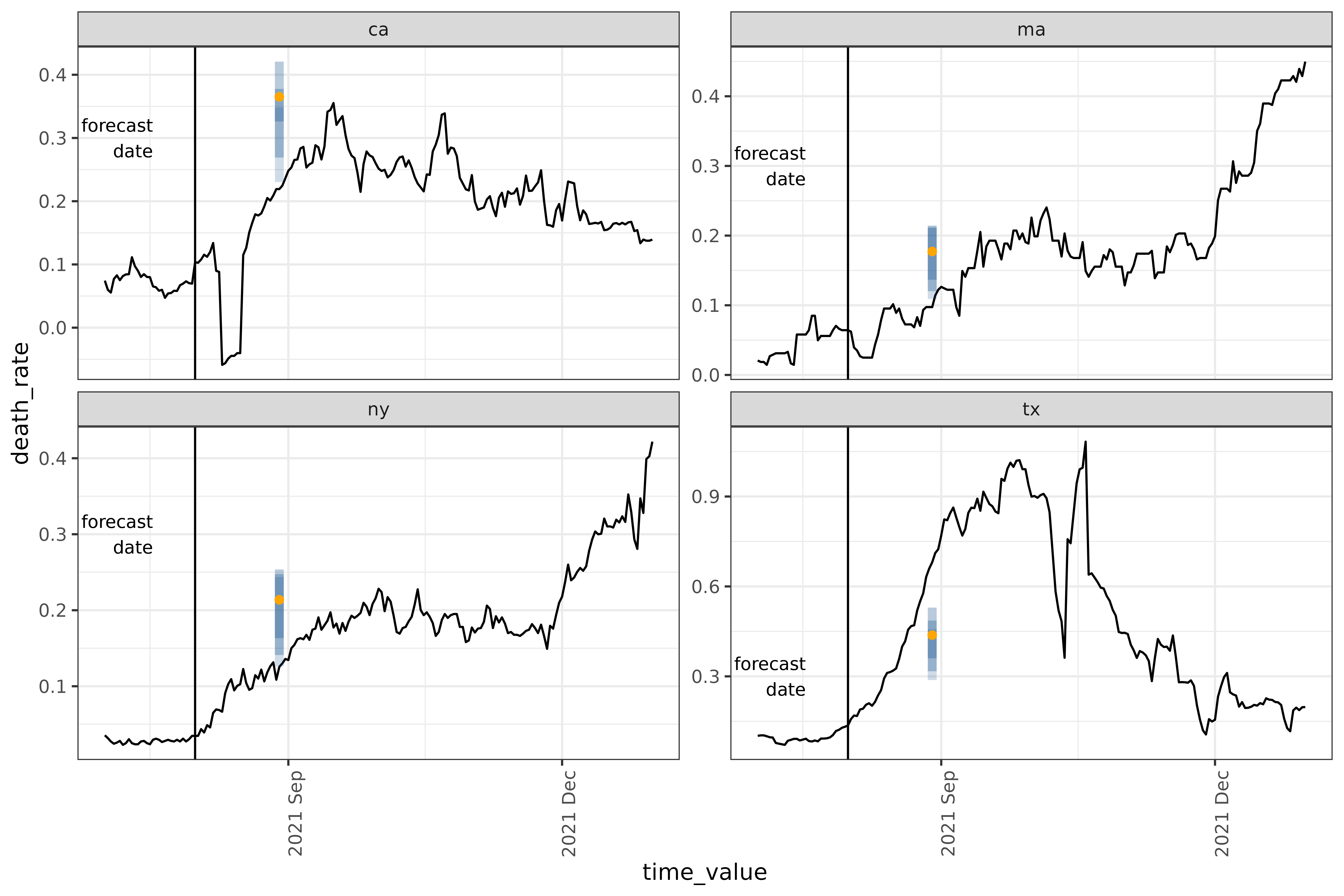
TODO get_test_data isn’t actually working here…
Population scaling
Suppose we’re sending our predictions to someone who is looking to understand counts, rather than rates. Then we can adjust just the frosting to get a forecast for the counts from our rates forecaster:
count_layers <-
  frosting() |>
  layer_predict() |>
  layer_residual_quantiles(quantile_levels = c(0.1, 0.25, 0.5, 0.75, 0.9)) |>
  layer_population_scaling(
    .pred,
    .pred_distn,
    df = epidatasets::state_census,
    df_pop_col = "pop",
    create_new = FALSE,
    rate_rescaling = 1e5,
    by = c("geo_value" = "abbr")
  ) |>
  layer_add_forecast_date() |>
  layer_add_target_date() |>
  layer_threshold()
# building the new workflow
count_workflow <- epi_workflow(
  four_week_recipe,
  linear_reg(),
  count_layers
)
count_pred_data <- get_test_data(four_week_recipe, training_data)
count_predictions <- count_workflow |>
  fit(training_data) |>
  predict(count_pred_data)
count_predictions
#> An `epi_df` object, 4 x 6 with metadata:
#> * geo_type  = state
#> * time_type = day
#> * as_of     = 2023-03-10
#>
#> # A tibble: 4 × 6
#>   geo_value time_value .pred .pred_distn forecast_date target_date
#>   <chr>     <date>     <dbl>   <qtls(5)> <date>        <date>
#> 1 ca        2021-08-01 135.        [135] 2021-08-01    2021-08-29
#> 2 ma        2021-08-01  11.3      [11.3] 2021-08-01    2021-08-29
#> 3 ny        2021-08-01  38.2      [38.2] 2021-08-01    2021-08-29
#> 4 tx        2021-08-01 117.        [117] 2021-08-01    2021-08-29
which are 2-3 orders of magnitude larger than the corresponding rates
above. df represents the scaling value; in this case it is
the state populations, while rate_rescaling gives the
denominator of the rate (our fit values were per 100,000).
Custom classifier workflow
As a more complicated example of the kind of pipeline that you can
build using this framework, here is an example of a hotspot prediction
model, which predicts whether the case rates are increasing
(up), decreasing (down) or flat
(flat). This comes from a paper by McDonald, Bien, Green,
Hu et al3, and roughly serves as an extension of
arx_classifier().
First, we need to add a factor version of the geo_value,
so that it can actually be used as a feature.
Then we put together the recipe, using a combination of base
{recipe} functions such as add_role() and
step_dummy(), and {epipreict} functions such
as step_growth_rate().
classifier_recipe <- epi_recipe(training_data) %>%
  add_role(time_value, new_role = "predictor") %>%
  step_dummy(geo_value_factor) %>%
  step_growth_rate(case_rate, role = "none", prefix = "gr_") %>%
  step_epi_lag(starts_with("gr_"), lag = c(0, 7, 14)) %>%
  step_epi_ahead(starts_with("gr_"), ahead = 7, role = "none") %>%
  # note recipes::step_cut() has a bug in it, or we could use that here
  step_mutate(
    response = cut(
      ahead_7_gr_7_rel_change_case_rate,
      breaks = c(-Inf, -0.2, 0.25, Inf) / 7, # division gives weekly not daily
      labels = c("down", "flat", "up")
    ),
    role = "outcome"
  ) %>%
  step_rm(has_role("none"), has_role("raw")) %>%
  step_epi_naomit()
Roughly, this adds as predictors:
- the time value (via
add_role()) - the
geo_value(viastep_dummy()and theas.factor()above) - the growth rate, both at prediction time and lagged by one and two weeks
The outcome is created by composing several steps together:
step_epi_ahead() creates a column with the growth rate one
week into the future, while step_mutate() creates a factor
with the 3 values:
where
is the growth rate at location
and time
.
up means that the case_rate is has increased
by at least 25%, while down means it has decreased by at
least 20%.
Note that both step_growth_rate() and
step_epi_ahead() assign the role none
explicitly; this is because they’re used as intermediate steps to create
both predictors and the outcome. step_rm() drops them after
they’re done, along with the original raw columns
death_rate and case_rate (both
geo_value and time_value are retained because
their roles have been reassigned).
To fit a classification model like this, we will need to use a
parsnip model with mode classification; the simplest example is
multinomial_reg(). We don’t actually need to apply any
layers, so we can skip adding one to the epiworkflow():
wf <- epi_workflow(
  classifier_recipe,
  multinom_reg()
) %>%
  fit(training_data)

forecast(wf) %>% filter(!is.na(.pred_class))
#> An `epi_df` object, 4 x 3 with metadata:
#> * geo_type  = state
#> * time_type = day
#> * as_of     = 2023-03-10
#>
#> # A tibble: 4 × 3
#>   geo_value time_value .pred_class
#>   <chr>     <date>     <fct>
#> 1 ca        2021-08-01 up
#> 2 ma        2021-08-01 up
#> 3 ny        2021-08-01 up
#> 4 tx        2021-08-01 up
And comparing the result with the actual growth rates at that point:
growth_rates <- covid_case_death_rates |>
  filter(geo_value %in% used_locations) |>
  group_by(geo_value) |>
  mutate(
    # multiply by 7 to get to weekly equivalents
    case_gr = growth_rate(x = time_value, y = case_rate) * 7
  ) |>
  ungroup()

growth_rates |> filter(time_value == "2021-08-01")
#> An `epi_df` object, 4 x 5 with metadata:
#> * geo_type  = state
#> * time_type = day
#> * as_of     = 2023-03-10
#>
#> # A tibble: 4 × 5
#>   geo_value time_value case_rate death_rate case_gr
#>   <chr>     <date>         <dbl>      <dbl>   <dbl>
#> 1 ca        2021-08-01     24.9      0.103    0.356
#> 2 ma        2021-08-01      9.53     0.0642   0.484
#> 3 ny        2021-08-01     12.5      0.0347   0.504
#> 4 tx        2021-08-01     30.7      0.136    0.619
So they’re all increasing at significantly higher than 25% per week (36%-62%), which matches the classification.
See the tooling book for a more in depth discussion of this example.